We hope you enjoy our   Q&A  Online Excel Course /Reference Guide on business calculation situations you might encounter using Microsoft Excel. This short excel online training course  will offer possible solutions to many of these calculations  like percentage increases, mark ups, percentage variances etc . The aim is to help minimise mistakes when you are making important calculations, especially where any such mistakes might have a serious consequence.

Target users:

This question and answer online excel training course will be suitable for those who have  basic excel knowledge with using functions and building  formulas. If  some calculations  require knowledge of other functions or techniques, these will be clearly outlined as will the difficulty level of each solution. This  online excel training course can also be used as a  practical examples & solutions  complement  our online excel course- WorkPlace Excel.

Objectives of this Online Excel Course:

Many Excel users   throughout their career will need to use Excel to  perform calculations that express the  key operational metrics of their organization’s data .We want to be able to do that without embarrassing errors occurring. These will includes calculations like-   percentage increases,  variance percentage changes, applying discounts, rounding up figures etc.
In this  ‘solution type ‘ online excel course , we will  show the basic maths of the situation and then how to implement them  in Excel accurately and safety , helping you to avoid  making costly reputation errors in your analysis work.
Also this online excel course solutions will be here as a future reference point  when you come across any of these specific  problems in the future.

Time Required.

This  online excel  course on the Excel Look up situations  will take 3-4 hours.

• Calculate the performance in percentage terms to budgeted target.
• Percentage Variance calculation for Positive and Negative numbers
• Calculating a Percentage of  the Total Amount.
• Calculating and Applying  a % Increase
• Calculating and Applying % Discount
• Calculating a Running Total
• Divide by Zero Errors
• Rounding Calculations
• Rounding up and down Calculations
• Rounding Up and Down to the Nearest  Cent
• Round up to Millions etc for Financial Reports

How to create a basic Markup formula?
How to calculate percentage markup on selling price?
How to calculate the  Markup percentages  on Cost?

Calculate the performance in percentage terms to budgeted target?

Knowledge: Basic Excel. Knowledge of formulas and basic operators required.

How does the actual performance compare to the forecasted or budgeted target in percentage terms. Mathematically to achieve this, divide the budgeted target by the actual.  For example, if we budgeted to sell 100 laptops and we sold 60, then your performance percentage is 60% (60/100).

Don’t forget to  apply the  Percentage format.to your formula cells.

Calculating a Percentage of  Total Amount.

Knowledge: Basic Excel. Knowledge of formulas , basic operators and the ABS Function required.

We want to measure in percentage terms what each component part contributed to the overall total.

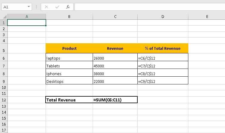
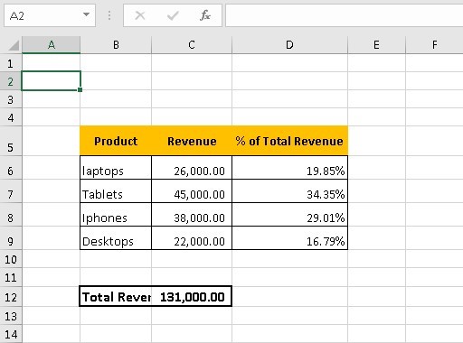
In our screenshot below , we  see the sales for each of our products and the total sales but  what is, for example,  the  laptop sales revenue  expressed as a percentage of the total sales etc.

To achieve this , we divide each product’s revenue by the total. The Excel formula for laptops would be =C6/C$12

 Warning:

Note cell C12 needs to be a partial absolute reference as we are copying the formula down , so the row element is locked.

Calculating and Applying  a % Increase.

Knowledge: Basic Excel. Knowledge of formulas , basic operators required.

To learn how to perform this  common calculation ,let’s take the following example. You need to apply  a 20%  increase to the price of a product as in the screenshot below .

So  we multiply the original amount by 1 plus the percentage of the increase. So we add 1 to the 20% , which gives 120%. You then multiply the original price of 200 by 120%. You then multiply the original price of 200 by 120%

The formula is  =D6*(1+E6)

Warning: 

Make sure you use parentheses, as we want Excel to do the addition first and then the multiplication. Without parentheses, multiplication would be done first, giving us the wrong answer.

Calculating and Applying % Discount

Knowledge: Basic Excel. Knowledge of formulas , basic operators required.

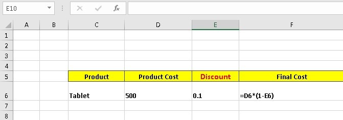
To apply a discount  to a product’s price, for example,  applying a discount of 10%  to a  product costing 500.  See screenshot below.

To achieve this , subtract the % discount from 1 and then multiply by the original amount.

So in our  example, we subtract  10% from 1 which gives 90% and multiply this by original price of 500.

The Excel formula is =D6*(1-E6)

Percentage Variance calculation for Positive and Negative numbers.

Knowledge: Basic Excel. Knowledge of formulas , basic operators and the ABS Function required.

A variance shows the difference between one value and another value.

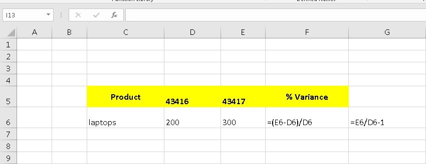
We sold 200 laptops yesterday and 300 today, so we sold 100 more laptops  today , so the difference in sales was 100 by simply subtracting 300 from 200 ( the anchor  number), giving a unit variance of +100

To see this as a percentage, we need to do the following calculation: Subtract the anchor number from the new number  and then divide the result by the anchor number. In our example,  the calculation would be

(300-200)/200=50%

So the percentage variance tells us that we sold 50% more laptops today compared to yesterday.

Warning:  
Note  the order of precedence in Excel. Division and multiplication are performed before addition and subtraction , so we need to use parenthesis  to force  Excel  to subtract  first , otherwise we  would get  an  incorrect answer. Putting the first part of the formula in parenthesis means Excel performs  this calculation first .

Alternative calculation method:

We  could also use this safer method of calculation instead.    =E6/D6-1

 Warning:
Another danger  occurs  if  dealing with negative numbers.  Let’s say that our benchmark  was  -200, so the calculation would be 300 minus -200 / -200 which is -250%.  This is definitely wrong as we have increased our sales. The maths here is inverting the result.

The solution is to use Excel’s ABS Function. The Excel ABS function returns the absolute value of a number. Negative numbers are converted to positive numbers, and positive numbers are unaffected.

So to get the correct result , the formula would now  be

=(E18-D18)/ABS(D18)

Calculating a Running Total.

Knowledge: Basic Excel. Knowledge of formulas , basic operators, partial references required.

Next in the online excel course, we will learn  the useful technique of creating a  running total of values.
This calculation can be done in Excel by using the SUM function  with a  partial reference.

The formula would be   =SUM(C4:C$4)

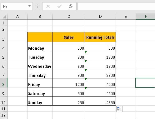
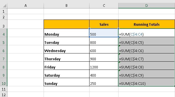
The key to the formula  is locking the first cell reference  so that it remains the same, while the second  C4 will change to C5, then C6 , C7 …etc as the formula is copied down.

Divide by Zero Errors.

Knowledge: Basic Excel. Knowledge of formulas , basic operators, partial references required.

In Excel as in mathematics, division by zero is impossible.
So in Excel , we don’t want such calculations to occur as it will only result in the #Div/0!  error  appearing.

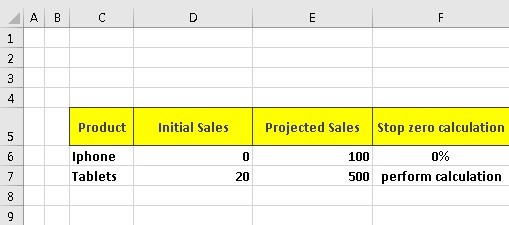
We can stop such calculations occurring by wrapping the calculation in an IF Function as in screenshots below.

The Excel formula is =IF(D6=0,0,(“perform calculation”))

The IF function tests the condition. If it’s true  i.e. cell D6 contains 0, then the IF function returns 0 but if cell D6 does not contain  0, then the calculation involving D6 takes places.

Rounding Calculations

Knowledge: Basic Excel. Knowledge of formulas , basic operators, Round Functions required.

To round a number is to eliminate the least significant digits, making your numbers  simpler and easier to comprehend  while  keeping close to the original values.

Microsoft Excel provides a number  of functions to handle the  different rounding situations you might encounter in your career using microsoft Excel.We will now look at some of these in our online excel course.

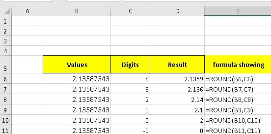
The Excel ROUND function returns a number rounded to a given number of digits. The ROUND function can round to the right or left of the decimal point.

=ROUND (number, number of digits to round to)

If the second argument is >0,  the number is rounded to the specified number of decimal places to the right of the decimal point. If negative, the number is rounded to the left of the decimal point (i.e. to the nearest 10, 100, 1000, etc.).

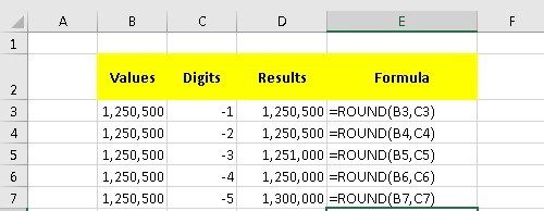
Let’s see some examples as in screenshots below

Let’s see some examples using negative numbers for the second argument. Think of this as rounding the integer number  to the  nearest 10, 100, 1000,10,000, 100,000, million etc

So to round a large number to the nearest million , use  -6 as the second argument.

If the number is 1,250,000  and the formula  used is =Round(1,250,000, -6)  it will  return a value of 1,000,000. If the number was 1,780,000 , the above formula would return 2,000,000

Let’s see some more examples.

Rounding up and Rounding down Calculations.

Knowledge: Basic Excel. Knowledge of formulas , basic operators, Round Functions required.

Often you need to force rounding in a particular direction. For this we can use the ROUNDUP or ROUNDDOWN functions.

The Excel ROUNDUP function returns a number rounded up to a given number of decimal places but  unlike the  standard rounding function  where numbers less than 5 are rounded down, ROUNDUP always rounds numbers 1-9 up.

So for example with the number 2.13587543, if we use the formula =ROUNDUP(B9,1), it will return the answer 2.2 , while the Round function would have returned 2.1.  Also ROUNDUP(67.45,0) returns 68

But on the other hand, the Excel ROUNDDOWN function returns a number rounded down to a given number of decimal places. Unlike standard rounding, where only numbers less than 5 are rounded down, ROUNDDOWN rounds all numbers 1-9 down.

So for example with the number 2.18587543, if we use the formula =ROUNDDOWN(B9,1), it will return the answer 2.1 , while the Round function would have returned 2.2.  Also ROUNDDOWN(67.45,0) RETURNS  67

Rounding Up  and Down  to the Nearest  Cent

Knowledge: Basic Excel. Knowledge of formulas , basic operators, Round Functions required.

Many times when making calculations in Excel, you will be required to round the amount to the nearest cent or penny. So now in our online excel course, we see we can achieve this calculation in Excel by using the CEILING or FLOOR Functions.

The Excel Ceiling function rounds a supplied number away from zero, up to the nearest multiple of a given number.

The syntax of the function is:

CEILING( number, significance )

The significance is the  multiple of significance that the supplied number should be rounded to.

Let’s look at  the calculation to round an amount up to the nearest cent.

We have amounts like 72.243 and we need to round them up to the nearest cent, the formula will be

=CEILING( 72.243,0.01) returning a value of 72.25

With 0.01 being the degree of significance for the nearest cent.

See the screenshot below.

The FLOOR Function works the same way except it causes a rounding down to the nearest significance, in this case to the nearest cent as in the screenshot example.

Round up to Millions etc for Financial Reports

Knowledge: Basic Excel. Knowledge of formulas , basic operators, ROUND, INT and  LEN Functions  required.

Financial reports figures are  expressed normally in terms of millions, tens of thousands etc. Now to make the report clearer to use , we don’t need to present the users with  superfluous numbers .

For example, if  we have a figure like 383,978, you could choose to round the number to one significant digit, thus the number  in the report would be displayed as 400,000. Rounding it to 2 significant digits would result in  380,000

But what if some of the numbers in your financial report are in millions, some in hundreds of thousands, you wont want them all rounded up to one significant digit.

Instead of having to create individual formulas for each number, we will build a formula which will automatically choose the correct level of significance.

See the screenshot below.

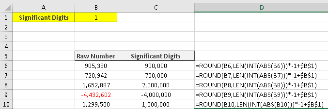
Remember from our previous rounding calculations, that the second argument in the ROUND function is the digit of significance. But instead of hard coding this figure   into our ROUND formula, we can create this figure on the fly.

To do this, we will use the INT function and the ABS function which we learnt about at the beginning of this solution based online excel course.

The formula would be

=ROUND( B6,LEN(INT(ABS(B6)))*-1+$B$1)

where we are using cell references for the values.

To see the formula  using actual  numbers it would be

=ROUND(720942.162347006,LEN(INT(ABS(720942.162347006)))*-1+2)

How does this formula work?.

Firstly, its important to know that Excel always evaluates from the  inner function outwards.

Quick Tip:

( Also note if you select a function and its arguments and press Function F9, Excel will return the value of the function.)

The ABS returns positive value of the number. This is needed if the number was negative. The INT function just returns integer part of the number and the len functions counts it’s length. So this formula would return  6 . This is then multiplied by -1 to make it a negative number , making it -6 and then this is added to the number of significant digits you are looking for , so its

6*-1+2=-4

This -4 will then become the second argument in your round function but it was calculated on the fly and not just hardcoded into your ROUND Function.

How to create a basic Markup formula?

Knowledge: Basic Excel. Knowledge of formulas , basic operators required.

How can you create a basic Markup formula? Well that’s what you will learn next in this online excel course.

The basic formula is  €Cost + €Markup = €Sell Price.

That is you add the markup amount to the cost of  the item to get the selling Price.

See screenshot examples below

How to calculate percentage markup on selling price?

Knowledge: Basic Excel. Knowledge of formulas &  basic  math operators required.

The next calculation in our online excel course on Excel calculations is  how can I calculate  the Markup percentages on selling prices?
Below we have a markup on selling price  calculator.

It is based on the  basic formula  of Markups which is is  €Cost + €Markup = €Selling  Price

That is  you add the markup amount to the cost of  the item to get the selling  price but this time the base is the selling price. It is 100% and the relationships are expressed in relation to selling price.

How to calculate the  Markup percentages  on Cost?

Knowledge: Basic Excel. Knowledge of formulas &  basic math operators required.

The next calculation in our online excel course on Excel calculations is how can you calculate  Markup percentages on Cost?
Below we have a markup on cost calculator.

It is based on the  basic formula  of Markups which is is  €Cost + €Markup = €Sell Price

i.e is you add the markup amount to the cost of  the item to get the selling Price.

So for example, the markup  in percentage terms is visible  as you change the actual Markup amount. As this calculator is based on cost,  cost is the base amount.