Online Excel Course Look Up Situations in Excel

We hope you enjoy our   Q&A  Online Excel Course /Reference Guide on Look-up situations you might encounter using Microsoft Excel. This short excel online training course  will offer possible solutions to many of these situations that might arise . See if you can work out a solution and then check it against ours.

Target users:

This question and answer online excel training course will be suitable for those who have learnt how to create  basic Vlookup, Index and Match functions. If  some solutions require knowledge of other functions or techniques, these will be clearly outlined as will the difficulty level of each solution.
This  online excel training course can also be used as a  practical examples & solutions  complement  our online excel course- WorkPlace Excel.

Objectives of this Online Excel Course:

To deepen your knowledge of looking up values in Excel from lists and tables  in many  various  circumstances. Also to act a future reference point  if you come across any of these specific  problems in the future. Look out for our upcoming article on the new XLOOKUP function , which will cause quiet a stir.

Time Required.

This  online excel  course on the Excel Look up situations  will take 2-3 hours.

• When adding a new record to my lookup table, I am getting an #N/A Error?
• I don’t want my Vlookup to return #N/A errors but another messsage?
• Can’t use a Vlookup function , as I need to search from right to Left ?
• How to Look up Multiple Index columns in a list?
• How to Look up a Value based on Column and Row ?
• Looking-up a number with decimal places but from right to left in your list?
• How to Look up a combined Text and Number column?
• How to Look up a Text and Number columns in Excel using Arrays?
• How do I lookup text that is case sensitive?
• How to lookup text that is case sensitive using Sumproduct?
•  How to search for text containing certain characters using the Lookup functions?
•  How to look up a Date using the Vlookup Function?

Basic level: Knowledge of Vlookup required.

Let’s start off  our online excel course on the  Vlookup function by solving a common problem that often occurs with this function. Look at the  example below.

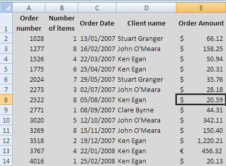
My lookup table is F2:G7. This is a table of product codes and what each code  stands for. In the B column, I need Excel to tell me what each of the product codes in in A2:A8 stands for. To achieve this I created the following VLOOKUP Function in  cell B2.

=VLOOKUP(A2,$F$1:$G$7,2,FALSE)

But then, a new product code has been created – code-106 , so I add it to my Lookup table in F8 and G8.

But yet when I type  106 into A9 and copy the down the VLOOKUP Function  into B9, I am getting the #N/A.

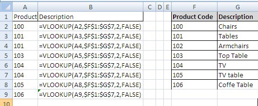
How can I fix  this problem. You  have the following solutions.

1. Redefine your lookup table in the VLOOKUP Function, to $F$1:$G$8
2. Insert the new row for 106 product details  within  your lookup table. This shifts the remaining items down and automatically expands the Vlookup range.
3. Specify F:G as the lookup table. This uses the whole column as the lookup table. Use this method with caution.
4. Use an Excel table to hold your data.  This would be by far our preferred solution

I don’t want my Vlookup to return #N/A errors but another messsage?

Basic level but requires the  use of the IFERROR Function

Often the appearance of  #N/A errors  makes a workbook appear as if it has lots of unintentional errors. But your workbook will  look more professional if we could replace these error symbols with  some other term.

This is how we do this.

IFERROR(VLOOKUP(Value, Dataset,Column No,FALSE), “- “)

The IFERROR Function is great for this. If the Vlookup function can return a correct value it will, but if it is returning an error like the N/A error, the second argument of the function is outputted instead. In this case , it will show the – symbol.

But it is important , that you make sure that  your Vlookup function is working correctly before  you place it inside the IFERROR Function as you don’t want it to hide any real errors.

Can’t use a Vlookup function , as I need to search from right to Left ?

 Advanced  level:   Knowledge of  Index & Match Functions.

This Q&A in our  Online Excel Course  you will soon come across as you get heavier into using Microsoft Excel.

The VLOOKUP Function search the left most column of your defined table and bring back values to the right of it. But what can you do , if the value you are searching is , for example, in the middle of your table and you want to bring back data to the left of it.

In these situations we need to use the INDEX and MATCH Functions.

An Example:

We have data in the Worksheet called ‘Data” that we want to look up and bring back an attribute from a specific record. See screenshots below. 

For example, In Cell G20, by inputting an ID, we want to bring back the Name and phone number for that ID.  But look at the first screenshot  below and notice that the user names are  to the right of the ID numbers. So we cant use a Vlookup function. We will get around this by using the INDEX AND MATCH Function.

The formula will be

=INDEX(Data!$A$16:$E$27,MATCH(G20,Data!$B$17:$B$27,0),1)

We know the table we want to search– Data!$A$16:$E$27 . We know that the name  we are searching for will be somewhere in the first column. The unknown factor  is what row the record we are searching is on. Thus we can use the MATCH Function, which returns the relative row position of that record.

 Note that the MATCH FUNCTION  can only search a column not a table. Give it a Table as the second argument, and it will return an error.

How to Look up Multiple Index columns in a list?

Very Advanced level:   Knowledge of Array formula, Index  & Match Functions required.

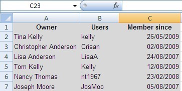
Lets look at an example to see this more clearly. Here is our sample dataset.

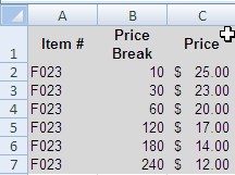
Our problem is that we need to be able to search for both the Item Number and the quantity ordered , to return  the Price Break, as show below.

The solution to this requires  an array Formula .

{=INDEX(Data9!$A$2:$C$7,MATCH(1,(Data9!$A$2:$A$7=B21)*(Data9!$B$2:$B$7>=C21),0),3)}

MATCH(1,(Data9!$A$2:$A$7=B21)  causes  the creation of a temporary array of {F023,FO23,F023,FO23,F023,FO23,F023} . This is evaluated against  the value in cell reference B21 which results in an arrays of {True…..True}.

This is multiplied by an second array which is  {10 30 60 120 180 240}<=C21  which depending on the value of B21 could end up as
Match(1,{1;1;1;0;0;0;0}

Remember in Excel False  =0 and True=1

The MATCH Functions then finds the location of the first 1 and this is then fed into the INDEX function.

How to Look up a Value based on Column and Row ?

 Advanced level:   Knowledge of  Index  & Match Functions required.

Lets look at an example.

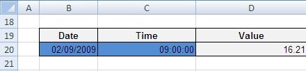
We want to be able to input a date into Cell B20  above and also input a time into Cell 20,and have a resultant value from the dataset below show up in cell D20.

But there is a complication, as you can see from looking at our list  below.

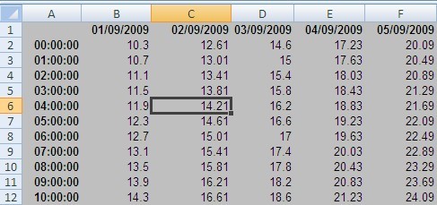
If we were doing this manually using our fingers, we would be  searching across  row 1   for the date and then  down  t column  A for the time, in order to return  the intersecting cell.

The formula we will use in cell reference  D20 will be

=INDEX(Data8!$A$1:$F$12,MATCH(C20,Data8!$A$1:$A$12,0),MATCH(B20,Data8!$A$1:$F$1,0))

This simply uses  two  Match  Functions  to find both the Row and Column data for the INDEX  Function.

So for example

MATCH(C20,Data8!$A$1:$A$12,0)

This function is saying ..Look for the value in cell C20, which is 9:00 and search for it in the single range A1:A12 and for that value exactly and if you find it, tell me its relative row postion. This is repeated for the date and both relative row positions now fill the index function.

Looking-up a number with decimal places but from right to left in your list?

 Very Advanced level:   Knowledge of  Array formula, Index  & Match  and Round  Functions  required.

This Question and Answer in our online excel course is actually quiet advanced.

Here is an example of this situation.

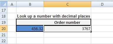
When we type in an order amount like 456.32  in cell B20, we want its  order Number to be shown in cell C20.

Now from looking at the dataset above,  there is an added complication –  the order amount in  column E and the  order number is in  column A.  Thus we will be  searching from right to left and can’t therefore use  the Vlookup function directly in the solution.

We will need to use the INDEX and MATCH Functions  so the formula we have used in cell C20 is

{=INDEX(Data5!$A$2:$E$14,MATCH(B20,ROUND(Data5!E2:E14,2),0),1)}

We also need the  the ROUND Function  in this formula. As you will have learnt in our WorkPlace Online Excel Course, the ROUND  function rounds a number to a specific number of digits.
We use Round on the numbers in the data range  E2:E14  so that 456.32335 becomes 456.32 etc etc

Also note that since we need to find the Round of all the values in the range E2:E14, we will need to use an ARRAY Formula. This as we have seen from previous example above  , will create a series of 1 and 0 or true or false

Look out for these important points.

1.  Use .025 instead of the 2.5%
   2.  Remember the number you see on the screen is not necessarily the number Excel deals with. e.g.  4.14 might be 4.139
   3. Array formula must be entered by using CTRL+SHF+Enter

How to Look up a combined Text and Number column?

 Intermediate  level:  Vlookup , helper column and the Concatenate Function

We want to Look up a Text and a Number from two index columns. In this example in our online excel course, we will use a very useful  technique called ‘Helper Columns”

Lets look at an example:

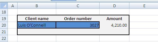
We want to be able to input a customer name in B20 and their order No In C20.

Then we want to bring back the amount for that order.

This is a common situation in Excel  especially since the Lookup functions cannot  handle duplicate values.

if there are two ‘Luis o’Connell’, it will only find the first occurrence of it.

The data set we will use is

To use this method, we create a add a new column to our data table . We have done this in the range  A2:A12 , as above , using the
formula  =B2&C2 and then copying it down.

Then we can use the VLOOKUP formula

=VLOOKUP(B20&C20,Data4!$A$2:$F$12,6,0)

Also note instead of using the & operator  ,  we can use the Concatenate Function instead

 =VLOOKUP(CONCATENATE(B20,C20),Data4!$A$2:$F$12,6,0)

How to Look up a Text and Number  columns in Excel using Arrays?

 Very Advanced level:   Knowledge of  Array formula, Index  & Match  and also the SumProduct function (optional) required.

This next Q&A in our online excel training course is also quiet advanced as it again uses array formulas and also can use the Sumproduct function as another  possible solution.

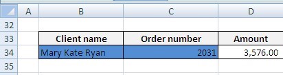
In this example, we want to be able to input a customer name like Mary Kate Ryan into cell  B34 and have her  Order Number  to be shown up  in cell C34. Finally we want the amount for that order to show up  in cell D34.

A sample of the dataset containing  the data is here.

This is a common problem that occurs in Excel  especially  also as the look up functions cannot handle  duplicate values.

If there are two ‘Mary Kate Ryans’, they  will only find the first occurrence of it.

The formula we will use in D34 is

{=INDEX(Data4!$A$16:$E$26,MATCH(1,(Data4!$A$16:$A$26=B34)*(Data4!$B$16:$B$26=C34),0),5)}

As an array formula ,this formula is based on creating a series of TRUES and FALSES  in   Data4!$A$16:$A$26=B34 and in  Data4!$B$16:$B$26=C34

This create two   series of 1 and 0 ranges.  Then  a True by True or 1 * 1 creates a 1 which the MATCH Function then searches for.

Once it finds the relative Row Position of this 1,it feeds  this  into the Index Function which then returns the correct attribute of the record been  looked for.

Alternative method using the  SUMPRODUCT :

You could use the SUMPRODUCT Function also. If we assume the customer’s name is inputed into B27, then we could use the following formula.

If you use or have used  our  Workplace online excel course , the Sumproduct function module shows how it also creates a array of values -1 or 0

=SUMPRODUCT((Data4!$A$16:$A$26=B27)*(Data4!$B$16:$B$26=C27)*Data4!$E$16:$E$26)

How do I lookup text that is case sensitive?

 Very  Advanced level:   Knowledge of  Array formulas and the Exact Function required.

This next Q&A in our  excel course online  is also quiet advanced as it uses  array formulas again.

We want to look up text that is case  sensitive.  We can’t use VLOOKUP , Index & Match because they are not  case sensitive. The solution  requires the use of   arrays.You may need to read  our module from our   online excel courses  on ‘ Array Formulae’  or  one from YouTube on array formulas to understand this task.

Let’s look at an example:

We want to search for Kelly and then kelly without a capital k as shown below.

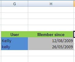
Here is the dataset we will be looking up:

The  formula in C20 is

{=INDEX(Data3!$A$2:$C$7,MATCH(TRUE,EXACT(Data3!$B$2:$B$8,B20),0),1)}

What is going on in this formula. We are going to use an array formula and the Exact Function to lookup case sensitive text.  The EXACT  function checks whether two text strings are exactly the same. It returns  True or  False and is case sensitive.

The Exact function will compare  the value in B20 to the values in B2:B8 in  our list . Sine it is an array formula it will return a series of  False values  and one True.

Then the Match function  will search for  the True and when it finds the True it will return it’s relative row position. This is then used in the INDEX Function to return the correct  attribute of the record. Remember when entering an array formula, use Ctrl+Shift+Enter

How to lookup text that is case sensitive using Sumproduct?

  Advanced level:   Knowledge of  the SumProduct function.

This next Q&A in our online excel course is also quiet advanced as it uses  the Sumproduct function

We want to look up text that is case  sensitive.  We can’t use VLOOKUP because it is not case sensitive.
We will use  the SUMPRODUCT Function to achieve our task.

Let’s look at an example: 

We want to search for Kelly and then kelly without a capital k as shown below.

Here is the dataset we will be looking up:

The Formula we are using in cell H20 is:

=SUMPRODUCT((EXACT(Data3!$B$2:$B$7,G20))*Data3!$C$2:$C$7)

How does this formula work?

The EXACT  function checks whether two text strings are exactly the same. It returns  True or  False and is case sensitive.
The Exact function will compare  the value in G20 to the values in B2:B8 in our dataset  This will  return a series of  0 ‘s and one 1.

Thus we are left with an array of  True and False values  multiplied by  the array of C2:C7. As in all array situations, the first element of the first array  acts against the first element of the second array, then the second element against the second, etc.

So we are left  with a series of True and false values  or 0 and 1.  And from this the  mathematical calculations are made  – 0 times any value is 0 and 1 times any value is that value.

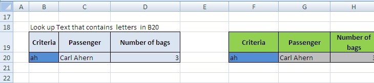
How to search for text containing certain characters using the Lookup functions?

  Intermediate  level:   Knowledge of  Vlookup  function and the & operator.

This Q&A in our online excel course is very a common problem that often arises when using Excel.

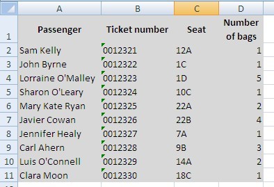
So this is the situation.  We want to look up records that  Begins/Ends/Contains  certain text.  So  cell B20 is our input cell. Cell C20 will bring back the passenger name that contains the letters ‘ah’. D20 will bring back that customer’s number of bags .

The list  that is been searched is

The formula in cell C20  is

 =VLOOKUP(“*”&B20&”*”,Data2!$A$2:$D$11,1,0) 

It uses  the &  text operator . This joins text together. We use it with the * symbol, which stand for any series of characters   or  you could hardcode it with  * beginingletters  and  end letters or use A5 if you put  beginingletters  *endletters into cell A5. The choice is yours.

Thus the VLOOKUP Formula is saying find a piece of text  that contains the letters ‘ah’ that has others letters before  and after it,  in the table located at A2:D11 .Then return the attribute in the first  relative column of that table and by the way,  only find an exact match (the final ’0′ argument)

The Vlookup function to bring back the number of bags is

=VLOOKUP(“*”&B20&”*”,Data2!$A$2:$D$11,4,0)

How to look up a Date using the Vlookup Function?

  Intermediate  level:   Knowledge of  Vlookup  and Date function and the & operator.

This Q&A in our  excel course online  is also a  very  common problem. What should you look out for when searching for a date when using the Vlookup function or the other Lookup functions.
In the example below, dates are associated with a phrase numbers so when  we inputted a date  into  Cell B26  , we want the phrase it is associated with to  come up in cell  C26

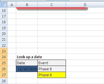
The Vlookup we will use in  C26 is

VLOOKUP(B26, Data!H1:J12,2,0)

where H1:J12 is the range that contains dates and their phrase numbers.

The important point to note is that we do not type in the date directly into the function.  typing in 12/10/2010 or “2/10/2010″ will not work.
Either use a cell reference ,like  B26 , as we have done or you can use the Date Function. So this formula is also correct

VLOOKUP( DATE(2010,10,12), Data!H1:J12,2,0)

Do not use dates directly in formulas.  12/10/2010 or “2/10/2010″ will not work. Use a Cell Reference as above or  DATE(2010,10,12)  or DATEVALUE(“2/10/2010″)

Other Useful Resources on Lookup Function.

The Hlookup Function 

A useful article from the knowledge team at the University of Wisconsin-Madison

Index & Match

A look at these functions from the Ohio State university